

A note on the format. Until now Macro Pulse was event driven. A number came out, we wrote about it. From this issue the format becomes monthly and quarterly.
The reason is that a single number misleads. It arrives without context, gets revised a month or two later, and rarely means what it appears to mean on the day it lands. This issue shows it well. Headline GDP says slowdown while private domestic demand accelerates. May payrolls were 172,000 on the first estimate and 129,000 on the second.
The point of the new format is direction, not event. Direction only becomes visible through repetition. One article on its own does little. Twelve in a row do a great deal.
This is the first quarterly issue.
I. Frame
This issue covers the second quarter of 2026 for the United States, meaning April, May and June. Every major release for the period is out. The last release included is the ISM Manufacturing PMI for July on 3 August 2026. July data enters only as a reading on the momentum carrying into the third quarter, not as part of the quarterly account.
II. Where the economy is
The phase is acceleration, and that is a change. For the previous two quarters the US economy sat in the most uncomfortable position available: domestic demand growth was weakening while inflation was accelerating. In the second quarter it left that position. Not because inflation calmed down, but because demand turned up.
Real GDP rose at an annual rate of 1.5 percent in the second quarter against 2.1 percent in the first. On the face of it that is a slowdown. Underneath the headline sits the other number BEA publishes in the same release: real final sales to private domestic purchasers, the sum of household consumption and private fixed investment, jumped to 3.9 percent from 1.7 percent in the first quarter. This is the measure of private domestic demand stripped of government, of inventories and of the distortion from imports. It more than doubled.
The engine is capital spending and consumption. Equipment investment is rising broadly, across industrial, transportation and information processing equipment at the same time. Intellectual property investment is rising in software and in research and development. Consumption accelerated in both goods and services. Imports confirm the same picture from the outside: the largest increases are in telecommunications equipment, semiconductors and industrial equipment, meaning goods that go into productive capacity rather than into consumption.
The brake is the labour market and the rate-sensitive sectors. Non-farm payrolls added just 57,000 jobs in June. Construction is contracting, and construction spending in the first half of the year was 3.5 percent below the same period of 2025.
The policy conclusion follows from there. Domestic demand growth is strengthening while headline inflation is accelerating. The PCE deflator rose 5.1 percent at an annual rate in the quarter against 4.6 percent in the first. Strengthening growth alongside accelerating inflation is the combination in which a central bank has no grounds to ease. The bias is towards tightening. On 29 July the Fed held rates, but three committee members voted to hike.
III. Core indicators
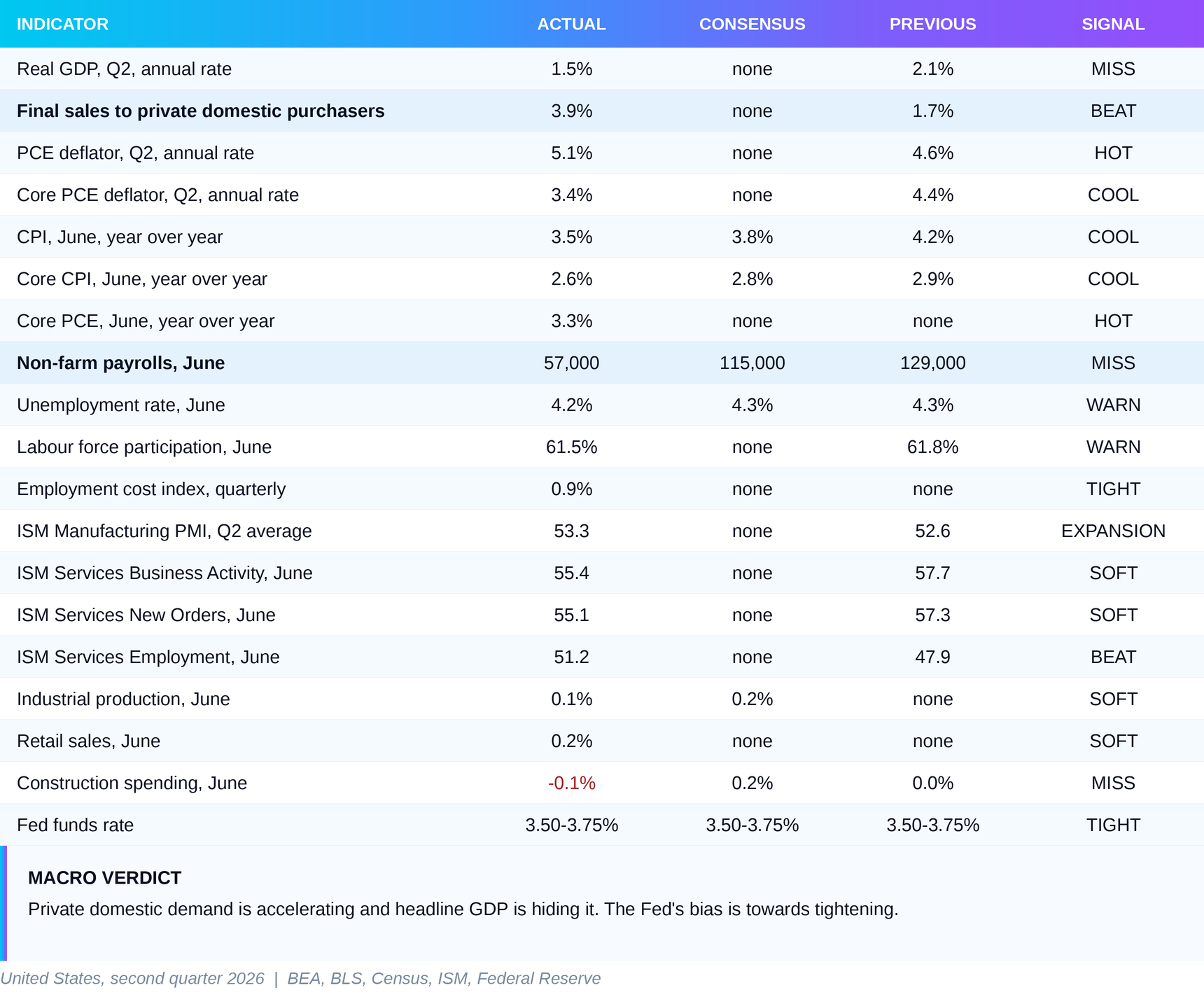
The WARN flag on the unemployment rate is an editorial judgement, not a mechanical one. Unemployment fell, but it fell for the wrong reason. The explanation sits in the section on the brake.
IV. The trajectory
The six months from January to June, with direction assigned by the format’s rule.
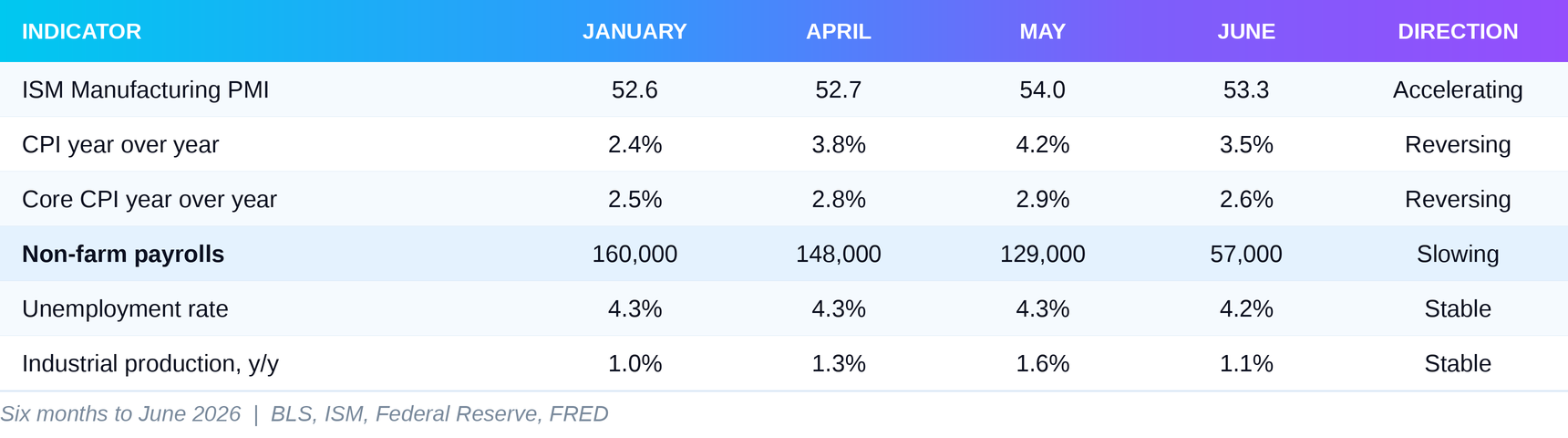
Three things in this table matter. The rest is context.
The first is the ISM. It is the only indicator in the core set that is accelerating under the strict rule: the current value sits above both the April and the January readings. The manufacturing sector is out of step with the rest of the economy, and that matters, because manufacturing is where the capital cycle shows up first. It is worth noting, though, that hard industrial production does not confirm the survey. It moves between 0.6 percent and 1.6 percent year over year across the whole half year and finishes at 1.1 percent, going nowhere. What is expanding is purchasing managers’ confidence, not necessarily the volume produced.
The second is the pair of inflation rows. Both reverse direction, which under the format’s rule is the most important case and always requires comment. The reversal is neither accidental nor a sign that underlying price pressure has calmed. Inflation climbed from 2.4 percent in January to a peak of 4.2 percent in May entirely because of energy, following the start of the conflict with Iran in March. The June ceasefire pulled the energy component down from a 15.7 percent annual rise from 23.5 percent, and headline inflation fell to 3.5 percent. The reversal is therefore a geopolitical event transmitted through petrol prices, not the result of demand contracting. The core measure reverses for the same reason, since energy enters core indirectly through transport costs with a lag of several months.
The third is payrolls. It is the only row in the table that deteriorates at every step, from 160,000 in January to 57,000 in June.
The conclusion from the trajectory is uncomfortable. Inflation improved for a reason outside the Fed’s control and one that can reverse within weeks. Meanwhile confidence in manufacturing is strengthening, the volume produced is flat, and employment is weakening. That is a divergence which usually resolves in one direction or the other within a quarter.
V. What pulled and what dragged
The gap between 1.5 percent headline growth and 3.9 percent growth in private domestic demand is about two and a half percentage points. Those points have not vanished. They sit in three places, and not one of them is contracting demand.
The first place is government. Government spending fell, with the decline led by federal nondefense outlays. The reason is an accounting one and deserves to be stated precisely, because almost nobody states it. During the quarter the government was selling crude oil from the Strategic Petroleum Reserve. In the national accounts, sales are deducted from government consumption, so more sales mechanically mean lower government spending. BEA notes explicitly that the oil sold shows up as an increase in other components of GDP and that there is therefore no direct effect on the headline. Put differently, part of the headline slowdown is a transfer between lines, not economic activity that disappeared.
The second place is imports. Imports rose, and imports are subtracted in the calculation of GDP. What matters is what was imported. The increase came mainly from capital goods excluding automotive, specifically telecommunications equipment, semiconductors and related devices, and industrial equipment. This is import that goes into productive capacity, not into consumption. It reduces measured GDP in the quarter it arrives and raises productive capacity in the quarters after. The arithmetic is counterintuitive: the more equipment an economy imports, the worse GDP looks now and the better it looks later.
The third place is inventories, and it deserves its own paragraph, because that is where the difference sits between durable growth and growth borrowed from the next period.
Private inventory investment fell during the quarter, with the largest contribution to the decline coming from wholesale trade. This is the opposite of the usual pattern, in which strong growth turns out to be stockpiling. Here domestic demand rose 3.9 percent while inventories were being drawn down. More was sold than was produced and stored. The economy did not borrow from the next quarter. It ate into its existing warehouses.
That has a direct consequence. If demand holds anywhere near current levels, firms will have to rebuild inventories, and rebuilding inventories enters GDP as a positive contribution. The third quarter therefore begins with a piece of built-in support that few people are talking about.
The rest of the picture is simpler. Consumption accelerated in both goods and services. Within goods the lead came from nondurables, mainly prescription drugs, followed by motor vehicles and parts, led by new light trucks, and furnishings. Within services the lead came from food services and accommodation, along with financial services and insurance, where portfolio management was the main contributor. Equipment investment rose broadly. Intellectual property investment rose in prepackaged software and in research and development. The only domestic investment component contracting was nonresidential structures, led by manufacturing structures.
Exports rose, but the composition is mixed. The increase came from goods, led by petroleum and related products, and was partly offset by a decline in services, led by travel and other business services.
VI. The quarter month by month
The averaged quarterly number hides the most important thing about this period. The second quarter was not even. It entered strong and left weak, and that is precisely what makes it hard to read.
Payrolls are the clearest case. April added 148,000 jobs, May 129,000, June 57,000. The quarterly average is about 111,000 a month, which is actually better than the first quarter, where the average was about 73,000 because of the loss of 156,000 jobs in February. So the second quarter was stronger than the first on employment and still finished with its own weakest month, with the decline clearly accelerating. Anyone looking only at the quarterly average sees improvement. Anyone looking at the monthly series sees free fall in the last two months.
Inflation runs the opposite profile. Annual inflation was 3.8 percent in April, 4.2 percent in May and 3.5 percent in June. The peak sits in the middle of the quarter. The June ceasefire with Iran brought energy prices down and the headline collapsed by 0.7 percentage points in a single month. The monthly reading for June was minus 0.4 percent, meaning prices fell in absolute terms.
Manufacturing runs a third profile. The ISM was 52.7 in April, 54.0 in May, 53.3 in June and then 55.6 in July. The middle of the quarter was stronger than its end, but July turns the movement back up with the strongest reading in four years. Industrial production year over year tells a more cautious story, moving from 1.3 percent in April through 1.6 percent in May to 1.1 percent in June.
The momentum carrying the economy into the third quarter is therefore contradictory. On labour it is negative, and that is the most serious signal in the entire account. On prices it is favourable, but for a reason that is not structural. On manufacturing it is positive and confirmed by the July data. The difference between reporting and analysis here is whether we say the quarter was decent, or that the quarter ended worse than it began. The second is the true one.
VII. The engine
The engine of the US economy in the second quarter is the capital cycle, supported by consumption that held up far better than expected.
The first question is how big the engine really is. Equipment and intellectual property investment together are about one eighth of the US economy, so on their own they cannot drive 3.9 percent growth in domestic demand. The number is therefore a combination: consumption, at roughly two thirds of the economy, accelerated at the same time as investment. Accelerating consumption alongside accelerating investment is rare and usually appears at the start of a cycle, not at the end of one.
The composition of investment says more than its size. Equipment growth is broad and spans industrial, transportation and information processing equipment. Intellectual property growth comes from prepackaged software and research and development. Imports confirm the same picture from the outside: the largest increases are telecommunications equipment, semiconductors and industrial equipment. This is the profile of building computing infrastructure. Companies are buying machines, chips and networking equipment, and paying for software and development.
The second question is whether the engine is durable or one-off, and it is the most important one. There are three pieces of evidence for durability.
The first is the behaviour of inventories. If the growth were pre-tariff front-running, inventories would be climbing, because front-run purchases get warehoused. Inventories fell.
The second is the composition of imports. Front-running shows up most often in consumer goods and in materials that can sit in a warehouse. Here the largest increases are telecommunications equipment, semiconductors and industrial equipment. These are long lead-time goods with multi-year lives, ordered against a production plan rather than against the expectation of a tariff two months out.
The third is that ISM new orders held in clear expansion, 56.8 in May and 56.0 in June. Here we should be precise: they weaken within the quarter rather than strengthen. This is the weakest of the three pieces of evidence and on its own it settles nothing.
Manufacturing employment does not help this argument during the second quarter. The index improved from 48.6 in May to 49.7 in June but stayed below fifty, meaning firms carried on shedding more than they hired. The only sector where employment crossed into expansion within the period was services, at 51.2 in June against 47.9 in May.
The third question is what would stop the engine. The answer is the cost of capital and the cost of inputs. The ISM prices paid index finishes the quarter at 73.0 in June, meaning raw materials have risen in price for a twenty-first consecutive month. If the Fed hikes while input costs stay at these levels, margins compress from both sides and capital plans get reviewed. The second risk is logistical. Supplier deliveries were deteriorating for a seventh consecutive month by the end of the quarter, and delivery delays are among the fastest in four years. A computing infrastructure project waiting on chips does not count as investment.
This is also where the structural theme on capital spending belongs, covered only in quarterly issues. US capital spending currently has an unusual shape. Equipment and intellectual property are growing while nonresidential structures contract for another quarter, led by manufacturing structures. Companies are buying machines but have stopped building the sheds to put them in. One explanation is that the factory construction wave of 2023 and 2024 has run its course and what was built is now being equipped. The other is that the high cost of long-term finance makes new construction uneconomic, while equipment depreciates faster and is easier to justify. The two explanations lead to different conclusions for 2027, and the data so far does not allow a choice between them.
VIII. The brake
The brake has two parts and they are different in nature. One is labour and it is largely structural. The other is the rate-sensitive sectors and it is purely cyclical. Conflating them is the main mistake being made in reading this period.
Start with labour. Non-farm payrolls added 57,000 jobs in June against expectations of 115,000. The May figure was revised down to 129,000, and April was also revised down by 31,000, to 148,000. The average for the twelve months before June is 36,000 a month. As raw numbers this looks like an economy that has stopped hiring.
Here comes the judgement on which the whole read depends. In June the unemployment rate fell to 4.2 percent from 4.3 percent. At the same time the labour force participation rate fell by 0.3 percentage points to 61.5 percent, its lowest since March 2021. Unemployment did not fall because people found work. It fell because people left the labour force and stopped being counted. The decline is not a one-off. Participation has fallen every month since the start of the year, from 62.1 percent in January through 61.9 percent in March to 61.5 percent in June.
This changes what 57,000 means. In an economy with shrinking labour supply, the number of new jobs required to hold unemployment steady also shrinks. If the labour force is contracting, even very weak job growth can be enough to stop unemployment rising. So 57,000 at 61.5 percent participation does not mean what it would mean at 63 percent participation. Weak employment in this period is at least partly a supply problem, not a signal that labour demand has collapsed.
The distinction has a direct practical consequence for monetary policy. Weak labour demand is disinflationary and justifies rate cuts. Shrinking labour supply is inflationary, because with fewer workers the wage for the same job goes up. The labour cost data supports the second. The employment cost index rose 0.9 percent for the quarter, which annualises to roughly 3.6 percent. Private sector compensation is growing at 3.3 percent year over year. This is not the behaviour of a labour market in collapse.
The two big business surveys tell a third story about the same period. The ISM services employment index moved back above fifty in June, to 51.2 from 47.9, meaning services firms are again hiring more than they are cutting. In manufacturing the index also improved, from 48.6 in May to 49.7 in June, though it stayed below fifty through the end of the quarter. So in the two largest sectors of the economy, hiring intent is improving in the same months in which the official count of new jobs falls from 148,000 to 57,000.
It matters to say what this does not prove. The ISM indices record how many firms are hiring and how many are cutting, not how many people. A firm that hired two counts the same as a firm that hired two hundred. So 51.2 and 57,000 cannot be reconciled arithmetically and nobody should claim otherwise. But the direction of both indices is up while the direction of the official count is sharply down, and that divergence is easier to explain by shrinking labour supply than by collapsing demand for it.
There is a flip side. Real wages, meaning wages after inflation, are falling 0.4 percent year over year in the private sector. Average hourly earnings are growing 3.5 percent, while inflation ran between 3.5 percent and 4.2 percent through the quarter, meaning it outpaced wages in April and May and only drew level in June. The working American is losing purchasing power while their employer pays them more. That is the definition of an inflationary labour market, not a disinflationary one.
The second part of the brake is purely cyclical and shows up everywhere the interest rate is decisive.
Construction is contracting. Construction spending fell 0.1 percent in June against expectations of a 0.2 percent rise. For the first half of the year, total construction spending is 3.5 percent below the same period the year before. Residential construction fell 0.3 percent in June. Within GDP itself, nonresidential structures are the only domestic investment component contracting, led by manufacturing structures.
This is also where the quarterly structural theme on real estate belongs. The thirty-year mortgage rate rose to around 6.69 percent, a high since August 2025. Building permits fell 2.6 percent to 1.374 million. Builder confidence on the NAHB index sits at 34 points, deep below the neutral level of 50. Housing starts jumped 19 percent to 1.427 million, but the increase came almost entirely from multi-family, which rose from 291,000 to 513,000, while single-family was unchanged at 895,000. The recovery in starts is therefore in rentals, not in ownership. New home sales rose 1.6 percent to 628,000, which is stabilisation at a low level rather than a turn.
This second part of the brake is cyclical because the mechanism is single and well understood: the price of long-term credit. It will loosen the moment long-term bond yields fall, and it will not loosen before that, regardless of anything else in the economy. The first part of the brake, shrinking labour supply, will not be loosened by an interest rate at all.
IX. Prices
The inflation picture in the second quarter splits into two incompatible halves, and the choice of which half to look at determines the entire policy conclusion.
The first half is the monthly consumer data and it is improving. Annual inflation fell to 3.5 percent in June from 4.2 percent in May, the first decline in five months and below forecasts of 3.8 percent. Core inflation fell to 2.6 percent from 2.9 percent, also below expectations. On a monthly basis consumer prices fell 0.4 percent, while the core reading was flat. The cause is clear and singular: energy. The annual rise in the energy index shrank to 15.7 percent from 23.5 percent after the ceasefire between the United States and Iran brought fuel prices down.
The second half is the quarterly deflators from the national accounts and they are deteriorating. The price index for gross domestic purchases rose 5.7 percent at an annual rate in the quarter against 3.6 percent in the first. The PCE deflator rose 5.1 percent against 4.6 percent. So on the measure that covers the whole economy rather than just the consumer basket, inflation accelerated in the second quarter, and materially so.
The two halves do not contradict each other. The quarterly deflators cover the whole period, including April and May when energy was at its peak. The monthly data for June captures only the end. The quarter as a whole was inflationary while its final month was disinflationary.
The gap between producer prices and consumer prices is the third mandatory element, and it demands more attention than the simple reading allows.
The ISM prices paid index finished the quarter at 73.0 in June. Any reading above 50 means prices rising, and 73.0 means rising sharply, for a twenty-first consecutive month by the end of the period. Five of the six largest manufacturing industries report price increases. Read as a level alone, this says producer costs are rising faster than the prices producers manage to charge their customers, and that pressure is waiting to be passed to the consumer.
The level is not the whole story, though, and the direction speaks more loudly. The index was 82.1 in May and fell to 73.0 in June. Nine points in a single month is a steep dissipation of cost pressure, and it moves in step with the retreat in energy prices after the ceasefire. The claim that pass-through is coming is therefore weaker than it looks from the absolute value alone.
Two outcomes follow rather than one. If the decline continues, the pressure dissipates before it reaches the shelf, and headline inflation in the autumn will follow energy down. If the decline stops around the June level, the less pleasant version stands: nearly two years of uninterrupted increases in raw material costs, which sooner or later comes out either in consumer prices or in margins, and margin compression shows up first in hiring and in investment. The data through the end of the second quarter does not allow a choice between the two.
Core PCE, the measure the Fed watches most closely, is 3.3 percent year over year in June. On a quarterly basis the core PCE deflator is 3.4 percent, an improvement on 4.4 percent in the first quarter but far above the 2 percent target. So even on the most favourable readable measure, inflation is more than a full percentage point above where the Fed wants to see it, and that is after the energy shock has already begun to dissipate.
X. The detail being underpriced
The sale of oil from the Strategic Petroleum Reserve entered the GDP account as a fall in government spending.
That sounds like an accounting footnote, and that is exactly why it goes unnoticed. The mechanics are as follows. When the government sells oil from the reserve, the sale is deducted from government consumption in the national accounts. So the more oil the Department of Energy sells, the lower federal spending appears. BEA says this in plain words in the technical notes to the 30 July release: the fall in government spending was led by federal nondefense outlays, and the pattern of nondefense spending primarily reflects sales of crude oil from the Strategic Petroleum Reserve.
The significance is twofold.
First, it changes how the 1.5 percent should be read. The media reading of the quarter was a slowdown driven by shrinking state spending, which is usually interpreted as fiscal tightening. It was not fiscal tightening. The government did not stop spending. It sold an asset, and the sale was recorded with a minus sign against outlays. BEA itself notes that the oil sold appears as an increase in other components of GDP and that there is therefore no direct effect on the headline.
Second, this has an end. The Strategic Petroleum Reserve has fallen to around 311.4 million barrels, its lowest in 43 years. A reserve already at a 43-year low cannot be sold down much longer. The mechanical negative contribution to government spending will therefore disappear, and when it does, the same effect flips to positive. If sales stop in the third or fourth quarter, the government component will appear to recover without the government having changed anything about its behaviour.
Anyone reading third-quarter GDP in October will see an acceleration and will look for a cause in demand. Part of the cause will be this.
XI. What this means
The monetary policy conclusion does not follow from growth on its own. It follows from growth and inflation together, because the same rate of growth means different things depending on whether prices are rising or falling. The map below sets out the four possible combinations and what each means for a central bank, with the last four quarters plotted on it.
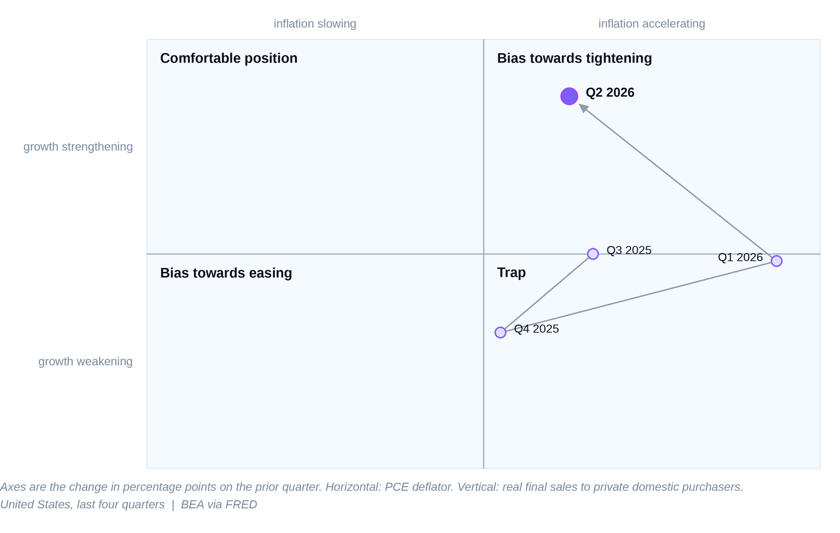
The second quarter puts the US economy in the tightening quadrant. Private domestic demand growth is strengthening, from 1.7 percent to 3.9 percent. Inflation on the broad measures is accelerating, with the PCE deflator moving from 4.6 percent to 5.1 percent. That combination has one conclusion and it is a bias towards tightening.
The value comes from where the economy was before. Across the last four quarters inflation has accelerated without interruption, meaning not one of those quarters lands in the left half of the map. In the third quarter of 2025 private demand growth was unchanged, and in the fourth quarter and the first quarter of 2026 it was weakening. So for two consecutive quarters the economy sat in the trap, where every decision carries a cost. A cut would have fed inflation, a hike would have hit already weakening demand.
The second quarter is the exit from the trap, and that is the news. The position remains uncomfortable, because inflation is still accelerating, but it is no longer a dead end. The central bank now has growth to lean on. That is also why three committee members voted for a hike on 29 July rather than two or none.
The Fed’s behaviour confirms the read. On 29 July the committee held the rate in the 3.50 to 3.75 percent range, but three members dissented, each voting for a 25 basis point increase. Three dissents in one direction are not noise. They are a minority convinced that policy is too loose. The statement was considerably shorter than usual, and Chair Kevin Warsh declined to give clear guidance on direction, stressing that the committee will not hesitate to act and that what matters is the direction of travel in the data rather than any single report.
From there follows what this means for liquidity conditions. The market entered the third quarter expecting rates on hold, with a non-zero probability of a hike. As long as that probability exists, long-term yields will not fall materially, and until they fall, the mortgage rate stays around 6.7 percent and the housing sector stays where it is. The cyclical part of the brake therefore has no mechanism to loosen over the next few months. Credit conditions for households remain tight even alongside solid growth.
For the ordinary person the picture splits like this. Anyone with a job keeps it but receives less in real terms: wages growing 3.5 percent against prices running 3.5 to 4.2 percent through most of the quarter, so purchasing power shrinks by roughly 0.4 percent year over year. Anyone looking for work will find it considerably harder than six months ago, because the monthly flow of new positions has fallen from close to 150,000 in April to 57,000 in June. Anyone wanting to buy a house is in the worst position in a year, with the mortgage rate at its high since August 2025. Anyone holding shares in companies building computing infrastructure is at the other end of the same economy.
Now the separation of what is confirmed from what is assumed.
The data already confirms the following. Private domestic demand is accelerating, and that is a measured number rather than an interpretation: 3.9 percent against 1.7 percent. Inventories are being drawn down, so the growth is not borrowed from the next period. Equipment and intellectual property investment are rising broadly. Inflation remains above target on every one of the four measures. The labour market is adding few jobs while participation shrinks.
The following remains assumption. That weak employment is primarily a supply problem rather than a demand problem. This is our thesis and it has only one quarter of evidence behind it. That the drawdown in inventories will lead to restocking in the third quarter. That the gap between producer and consumer prices will be passed to the consumer rather than absorbed by margins. And that the ceasefire with Iran will hold long enough for energy inflation not to return.
XII. What we said last quarter
This is the first quarterly issue, so the reconciliation is against the monthly material from the period. Three claims deserve checking.
The first was the thesis of jobless growth in manufacturing. In the May and June analysis we wrote that the manufacturing sector was expanding while the employment sub-index recorded the sharpest contraction in the workforce since May 2020, and we described this as a structural feature of the current cycle. Within the second quarter the thesis is not refuted, but it is weakened. The manufacturing employment index moves from 48.6 in May to 49.7 in June, so it continues to contract, but more slowly. At the same time services employment crossed into expansion, at 51.2 in June from 47.9 in May. Through the end of the period, jobless growth still holds in manufacturing but no longer holds for the economy as a whole.
We record the thesis as open rather than confirmed or refuted. The distinction between structural and cyclical is the central judgement in this format, and that is precisely why it is not settled by two months of data. If manufacturing employment holds above fifty through the third quarter, the thesis falls and we were wrong to have called something structural that was cyclical. The check is in the next issue.
The second was the expectation of weak consumption. In the July report we wrote that consumption was expected to stay sluggish, since real disposable income was growing just 0.3 percent while savings were shrinking. This turned out to be wrong. Consumption accelerated during the quarter and on BEA’s data was one of the three positive contributors to GDP, with real consumer spending rising 0.4 percent in June alone. Our error was methodological: we derived a consumption forecast from income dynamics without accounting for the fact that households can sustain spending through savings and credit considerably longer than the income arithmetic implies.
The third was more accurate. We wrote that strong regional manufacturing data suggested industry could lead the economy through the second half of the year, provided the geopolitical situation stabilised. The condition was met in June. We also correctly identified the energy component as the main driver of the inflation peak and said de-escalation would bring it down quickly. That is exactly what happened, and within a single month.
In summary: we were wrong in both of our negative expectations and right in the positive one. That is a pattern worth attention, because it suggests a systematic tilt towards pessimism in our reading of US data through the first half of the year.
XIII. The argument against our read
The strongest honest version of the opposing case looks like this.
The number working hardest against us is 57,000. Not the number itself, but the sequence: 148, 129, 57. Alongside it, April was revised down by 31,000 and May from 172,000 to 129,000. When a run of revisions moves in only one direction, it usually means the statistical model is failing to catch the turning point. History shows that successive downward revisions to employment are among the most reliable early signals of the start of a recession, and that they appear precisely when production and consumption data still look fine. If that is the case here, then 3.9 percent is the lagging indicator and 57,000 is the leading one, and we have classified the phase off the wrong one of the two.
The second mechanism that explains the same data involves tariffs. The acceleration in domestic demand may be front-running. Companies expecting higher tariffs or supply disruption buy equipment earlier. The July ISM report says exactly this, noting that manufacturing continues to benefit from businesses front-loading orders to avoid potential disruptions and higher costs. If that is a significant part of the 3.9 percent, then demand has not accelerated but has been moved forward in time, and the third or fourth quarter pays the bill. Our counter-argument that inventories are falling weakens on close reading: capital equipment is not recorded in inventories but directly in investment, so front-running equipment purchases would not show up as inventory accumulation.
There is also a hard number that supports this version. Factory orders rose 5.3 percent in April and reversed to minus 1.3 percent in May. A spike and a reversal in two consecutive months is the classic signature of front-running: orders move forward in time and the month after is left empty. If that is a significant part of the acceleration in investment during the quarter, then some of the 3.9 percent is borrowed and the bill falls due in the autumn. Working against this version is the fact that the survey data does not confirm it. ISM new orders were 56.8 in May and 56.0 in June, so purchasing managers are not reporting exhausted demand. The hard factory orders data and the surveys of purchasing managers tell different stories about the same thing, and at this point we have no grounds to prefer either.
The third argument is simpler. Domestic demand may have been flattered by one-off compositions. The leading contribution within goods came from nondurables, mainly prescription drugs. One of the leading contributions within services came from financial services, led by portfolio management, which tracks market levels rather than consumer behaviour. Neither is discretionary consumption and neither describes a confident household.
What would have to appear in the third quarter for us to be wrong. Three things at once. Payrolls staying below 75,000 a month through July and August with participation stable or rising, which would prove the problem is in labour demand rather than in supply. ISM new orders falling below 52, which would show that July’s strength was the last impulse of front-running. And the revised measure of final sales to private domestic purchasers being cut below 3.0 percent at the second estimate on 26 August.
If all three happen, the phase is not acceleration and never was.
XIV. Risks in both directions
The downside risks are four and all are drawn from things already visible in the data.
The first is the return of the energy shock. The ceasefire with Iran is why headline inflation fell from 4.2 percent to 3.5 percent in a single month. The same mechanism works in reverse and at the same speed. The Strategic Petroleum Reserve is at a 43-year low, so the buffer for responding to a fresh disruption is smaller than it has ever been.
The second is a monetary policy error. Three members voted for a hike with payrolls at 57,000. If the majority joins them in September and weak employment turns out to be a demand problem rather than a supply one, the tightening arrives at exactly the wrong moment.
The third is the pass-through of producer costs. The ISM prices paid index finishes the quarter at 73.0 with raw materials rising for twenty-one consecutive months. If the decline stops and the pressure is passed to the consumer in the autumn, inflation rises again without a fresh energy shock.
The fourth is weakness spreading outward from construction. The sector is contracting 3.5 percent year over year for the half, and builder confidence sits at 34 points. Construction is labour intensive, and a prolonged contraction shows up in employment before it shows up anywhere else.
The upside risks are three and they are not a courtesy.
The first is inventory rebuilding. Inventories fell while demand accelerated. If demand holds, restocking enters GDP directly as a positive contribution in the third quarter.
The second is the base effect in inflation. Energy prices jumped sharply from March onward. If levels stay stable, the annual comparison improves automatically through the autumn, which could bring headline inflation down faster than the market expects without the Fed doing anything.
The third is the capital cycle. If the second quarter’s imports of semiconductors and telecommunications equipment are what they appear to be, meaning capacity building, the effect on productivity appears with a lag of several quarters. Productivity-led growth is the only kind of growth that does not create inflation.
XV. What to watch
July payrolls on 7 August. The threshold is a reading below 50,000 with participation no longer falling. That combination would prove the weakness is in labour demand, and the phase changes from acceleration to growth with slowing momentum.
July consumer inflation on 12 August. The threshold is core CPI above 2.9 percent. A return above the May peak would close the door on a cut for the rest of the year.
The second GDP estimate and corporate profits on 26 August. We watch whether final sales to private domestic purchasers stays above 3.5 percent after revision. Corporate profits appear for the first time for the quarter and are the structural theme missing from this issue.
July retail sales around 14 August. We watch the reading excluding petrol stations, because with fuel prices falling the headline understates real consumption.
ISM Manufacturing for August on 1 September. The threshold is new orders below 52, which would mean July’s strength was the last impulse of front-running.
Construction spending on 1 September. We watch whether the decline deepens after five months of contraction.
The Fed meeting in September. We watch whether the three dissenters become a majority.
XVI. Close
The US economy enters the second half of 2026 with stronger private demand than headline GDP shows, and a weaker labour market than its capital cycle would imply. The two cannot continue side by side for long.
What we do not yet know is which of the two is leading. If participation stabilises while hiring stays weak, then we have read the data wrongly and the slowdown is real. If participation keeps falling while investment keeps rising, then America is growing with fewer people, and that is an inflationary economy regardless of how good GDP looks.
XVII. Sources
Bureau of Economic Analysis, GDP (Advance Estimate), 2nd Quarter 2026, 30 July 2026. Bureau of Economic Analysis, GDP (Advance Estimate), 4th Quarter 2025, 20 February 2026. Bureau of Economic Analysis, Personal Income and Outlays, June 2026, 30 July 2026. Bureau of Labor Statistics, The Employment Situation, June 2026, 2 July 2026. Bureau of Labor Statistics, Consumer Price Index, June 2026, 14 July 2026. Bureau of Labor Statistics, Employment Cost Index, June 2026, 31 July 2026. Institute for Supply Management, Manufacturing PMI Report, June 2026, 1 July 2026. Institute for Supply Management, Services PMI Report, June 2026. U.S. Census Bureau, Full Report on Manufacturers Shipments, Inventories and Orders, May 2026. U.S. Census Bureau, Advance Monthly Retail Trade Report, June 2026. U.S. Census Bureau, Construction Spending, June 2026, 3 August 2026. U.S. Census Bureau, Advance Economic Indicators Report, June 2026. Federal Reserve, FOMC Statement, 29 July 2026. Federal Reserve, Industrial Production and Capacity Utilization G.17, June 2026. Federal Reserve Bank of St. Louis, FRED, series PB0000031Q225SBEA, PCECTPI, PAYEMS, UNRATE, CIVPART, CPIAUCSL, CPILFESL, INDPRO. Baha Economic Calendar.
Not financial advice.
Liquidity Desk | liquiditydesk.org